Perform Stability Clustering

Partitioning Around Medoids (PAM) is used both because is uses a more robust measurement of the cluster centers (medoids) and because this implementation keeps the cluster labels consistent across runs, a key feature in calculating the across run stability. This does not occur using kmeans() where the initial cluster labels are arbitrarily assigned.

Usage

stability_cluster(data, k, iter = 100)

Arguments

data: A (n x p) data matrix containing n samples and p features. Can also be a data frame where each row corresponds to a sample or observation, whereas each column corresponds to a feature or variable.
k: integer(1). The number of clusters.
iter: integer(1). The number of random subset iterations to perform.

Value

A n x (k + 1) dimensional tibble of clustering probabilities for each k, plus a final column named "ProbK", which indicates the "most probable" cluster membership for that sample.

Note

How do we make sure clusters are indexed the same as what comes out of k-means? Worried about index errors (but seems ok for now).

References

Hastie, et al. 2009.

Author

Stu Field

Examples

stab_clust <- withr::with_seed(999, stability_cluster(progeny_data, k = 3, iter = 500))
table(actual = rep(1:3L, each = 50L), predicted = stab_clust$ProbK)
#>       predicted
#> actual  1  2  3
#>      1 49  1  0
#>      2  0 46  4
#>      3  1  0 49

stab_clust$true_cluster <- rep(1:3L, each = 50L)

# View the stable clusters
stab_clust
#> # A tibble: 150 × 5
#>    `k=1` `k=2` `k=3` ProbK true_cluster
#>    <dbl> <dbl> <dbl> <dbl>        <int>
#>  1 0.718 0.156 0.126     1            1
#>  2 0.684 0.172 0.144     1            1
#>  3 0.682 0.152 0.166     1            1
#>  4 0.664 0.19  0.146     1            1
#>  5 0.642 0.184 0.174     1            1
#>  6 0.7   0.154 0.146     1            1
#>  7 0.696 0.13  0.174     1            1
#>  8 0.644 0.154 0.202     1            1
#>  9 0.652 0.178 0.17      1            1
#> 10 0.682 0.154 0.164     1            1
#> # ℹ 140 more rows

# View the incorrectly clustered samples (n = 6)
filter(stab_clust, ProbK != true_cluster)
#> # A tibble: 6 × 5
#>   `k=1` `k=2` `k=3` ProbK true_cluster
#>   <dbl> <dbl> <dbl> <dbl>        <int>
#> 1 0.37  0.442 0.188     2            1
#> 2 0.196 0.376 0.428     3            2
#> 3 0.228 0.346 0.426     3            2
#> 4 0.174 0.406 0.42      3            2
#> 5 0.162 0.388 0.45      3            2
#> 6 0.636 0.224 0.14      1            3

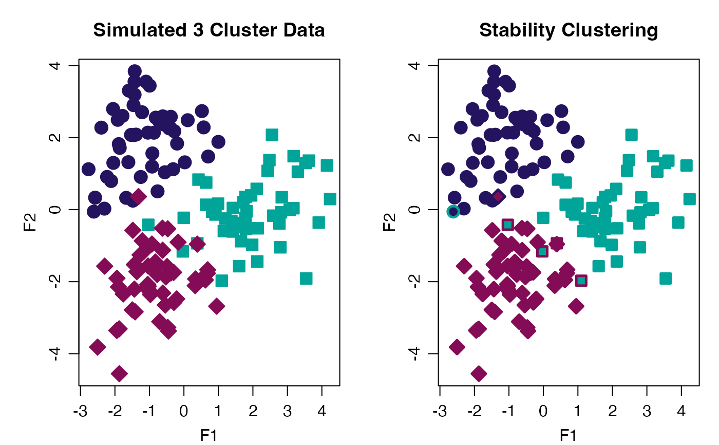
# Plot Stability Clusters
cols <- c("#24135F", "#00A499", "#840B55")
withr::with_par(list(mgp = c(2.00, 0.75, 0.0), mar = c(3, 4, 3, 1), mfrow = 1:2L), {
  plot(progeny_data,
       col = cols[stab_clust$true_cluster],
       bg  = cols[stab_clust$true_cluster],
       pch = stab_clust$true_cluster + 20,
       lwd = 1, cex = 1.75, main = "Simulated 3 Cluster Data")
  plot(progeny_data,
       col = cols[stab_clust$ProbK],
       bg  = cols[stab_clust$true_cluster],
       pch = stab_clust$true_cluster + 20,
       lwd = 2.5, cex = 1.5, main = "Stability Clustering")
})