Calculate Empirical Number of False Positives

Calculate the mean number of false positive features from a permutation analysis performed during a stability selection run. This assumes a permutation set was generated during stability selection, (i.e. n_perm > 0).

Usage

calc_emp_fdr(x, thresh_seq, warn = TRUE)

calc_emp_fdr_breaks(
  x,
  thresh_seq = seq(1, 0.1, by = -0.01),
  fdr_breaks = c(0.5, 1, 2, 3, 5)
)

plot_emp_fdr(x, ...)

plot_permuted_data(x, which = NULL, ...)

Arguments

x

A stab_sel class object generated via stability_selection().

thresh_seq

numeric(n). A sequence in [0, 1] specifying the thresholds. See thresh in get_stable_features()

warn

logical(1). Should warnings be triggered if mean of < 5 permutations is being returned?

fdr_breaks

numeric(n). A vector specifying the desired mean number of empirical false positives at which to calculate various thresholds.

numeric(n). A vector specifying the

...

Additional arguments passed to either calc_emp_fdr_breaks() (i.e. thresh_seq and fdr_breaks) or plot.stab_sel().

which

integer(1). Which of the null hypothesis permuted stability paths to plot.

Value

A named vector indicating the average number (counts) of false positive features selected at the various thresholds specified by thresh_seq.

For calc_emp_fdr_breaks(), a list containing:

n_selected: A vector of the number of features selected at each empirical stability selection threshold
meanFPs: A vector of the mean number of false positive selected features at each empirical stability selection threshold
breaks: A tibble of containing empirical false positive summary statistics at each FDR specified break point

Functions

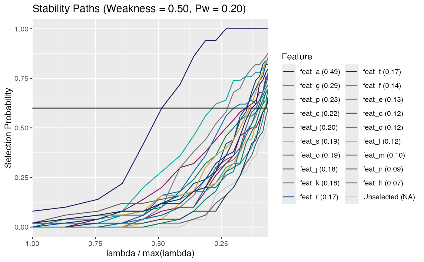
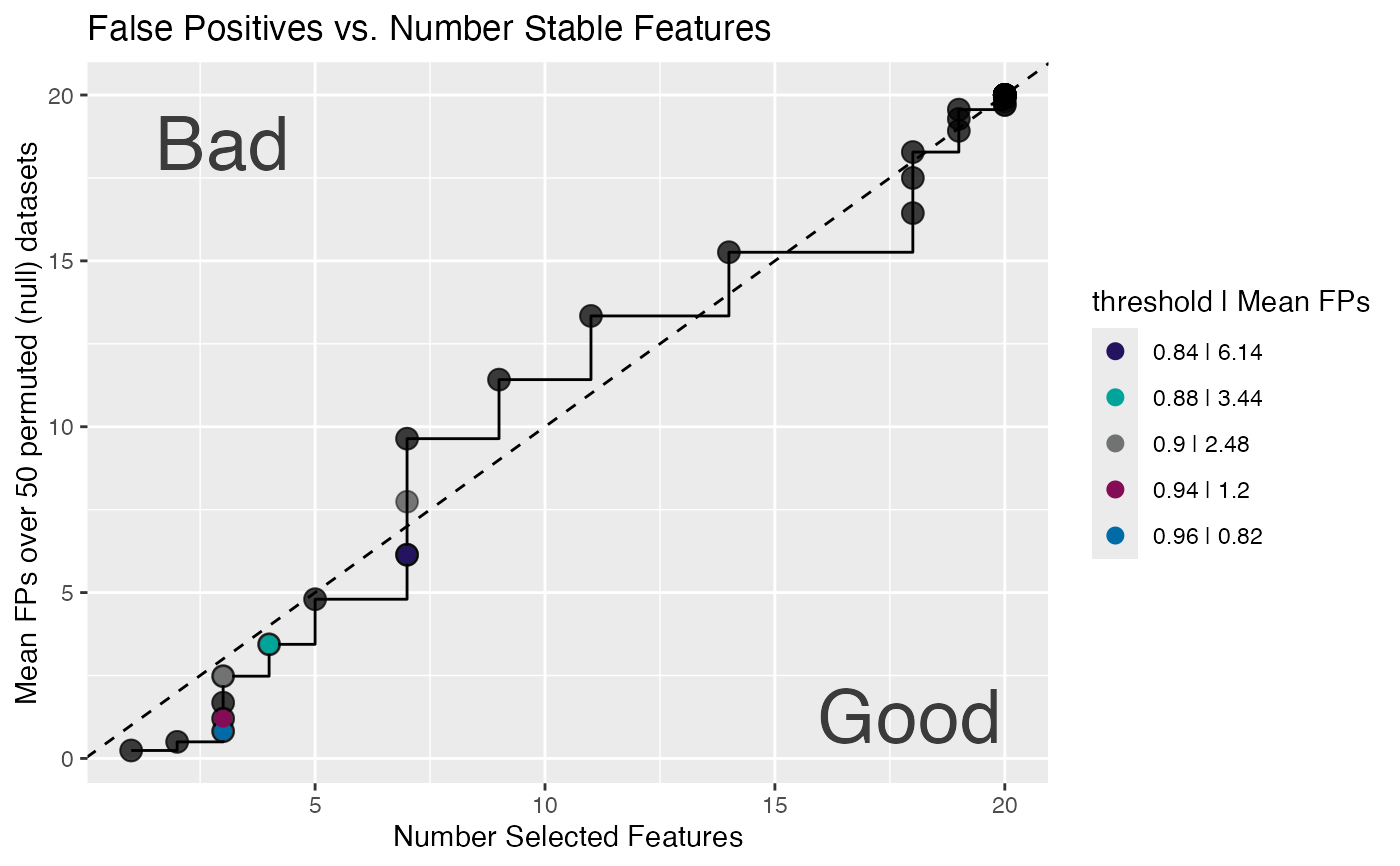
calc_emp_fdr_breaks(): Calculates the stability selection threshold, the mean number of false positive selected features (empirical), and the number of selected features for specified FDR break points. Relies on calc_emp_fdr() to calculate the mean false discovery based on permutations during the stability selection algorithm.
plot_emp_fdr(): plots the mean number of false positives (FPs) versus the number of selected features by a sequence of selection probability thresholds. For this to be possible, the stab_sel object must have permuted data in order to calculate empirical false discovery rates. The area in the sub-diagonal represents where more features are added without a commensurate increase in false positives (Good). The inverse is true for the super-diagonal, false positives are being included faster than additional features (Bad). The legend highlights pre-defined empirical FDR breaks: c(0.5, 1, 2, 3, 5) evaluated to the nearest threshold cutoff.
plot_permuted_data(): Plot the permutation paths for a stab_sel object. These paths are the stability selection paths of the n class scrambled permutations, i.e. the null.

Author

Stu Field, Michael R. Mehan

Examples

n_feat      <- 20
n_samples   <- 100
x           <- matrix(rnorm(n_feat * n_samples), n_samples, n_feat)
colnames(x) <- paste0("feat", "_", head(letters, n_feat))
y           <- sample(1:2, n_samples, replace = TRUE)

ss <- stability_selection(x, y, n_iter = 25, n_perm = 50,
                          r_seed = 101, parallel = TRUE)
#> ✓ Using kernel: 'binomial' and 1 core (serial)
#> ✓ Stablity path run time: 0.087s
#> ✓ Perm path run time: 2.723s

calc_emp_fdr(ss, seq(0.5, 0.9, 0.1))
#> thresh_0.5 thresh_0.6 thresh_0.7 thresh_0.8 thresh_0.9 
#>      20.00      19.70      17.50       9.64       2.48 

# calculate the FDR break points
calc_emp_fdr_breaks(ss)
#> $fdr_data
#> # A tibble: 91 × 3
#>    MeanFPs n_selected piThresh
#>      <dbl>      <int>    <dbl>
#>  1    0.24          1     1   
#>  2    0.24          1     0.99
#>  3    0.5           2     0.98
#>  4    0.5           2     0.97
#>  5    0.82          3     0.96
#>  6    0.82          3     0.95
#>  7    1.2           3     0.94
#>  8    1.2           3     0.93
#>  9    1.68          3     0.92
#> 10    1.68          3     0.91
#> # ℹ 81 more rows
#> 
#> $breaks
#> # A tibble: 5 × 4
#>   FDR_breaks MeanFPs n_selected piThresh
#>        <dbl>   <dbl>      <int>    <dbl>
#> 1        0.5    0.82          3     0.96
#> 2        1      1.2           3     0.94
#> 3        2      2.48          3     0.9 
#> 4        3      3.44          4     0.88
#> 5        5      6.14          7     0.84
#> 

# plot the FDR
plot_emp_fdr(ss)  # typically set permutations > 75


# Plot the permuted data individually
plot_permuted_data(ss, 3L)   # choose 3rd permutation