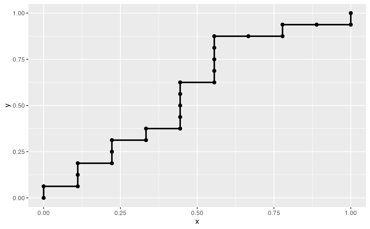
ROC Curve Coordinates

Calculate the the (x, y) coordinates of an empirical ROC curve.

Usage

roc_xy(truth, predicted, pos_class)

Arguments

truth

character(n) or factor(n). A vector of true class names. In most instances you will have to also pass a pos_class argument defining the positive/event class.

predicted

numeric(n). A numeric vector of class probabilities.

pos_class

character(1). Name of the "positive" or "event" class.

Value

A matrix containing the x and y coordinates for the ROC curve. A matrix is preferred over a data frame for speed of indexing while iterating over the rows and having to convert between classes. Downstream code will often convert to data frame while the main AUC functionality prefers a matrix.

Details

This algorithm was adapted from the one in Fawcett (2006) to account to a more accurate step calculation of indices with ties. The original paper suggests moving along the diagonal when tied according to the expected sensitivity and specificity, however this does not account for ties that occur within the same class, in which case a walk along the edge of the "unknown" box is the correct decision. In this algorithm, a step in the diagonal only occurs if there is a tie and the current class name differs from the previous. Otherwise, a full step occurs in the appropriate direction, up for positive classes, right for negative classes.

References

Fawcett, Tom. 2006. An introduction to ROC analysis. Pattern Recognition Letters. 27:861-874.

See also

plot_emp_roc(), create_roc_data()

Other ROC: calc_roc_fit(), create_roc_data(), geom_roc(), plot_boot_roc(), plot_emp_roc()

Author

Stu Field

Examples

n <- 25
withr::with_seed(22, {
  true <- sample(c("control", "disease"), n, replace = TRUE)
  pred <- runif(n)
})
xy <- roc_xy(true, pred, "disease")
xy
#>               x      y
#>  [1,] 0.0000000 0.0000
#>  [2,] 0.0000000 0.0625
#>  [3,] 0.1111111 0.0625
#>  [4,] 0.1111111 0.1250
#>  [5,] 0.1111111 0.1875
#>  [6,] 0.2222222 0.1875
#>  [7,] 0.2222222 0.2500
#>  [8,] 0.2222222 0.3125
#>  [9,] 0.3333333 0.3125
#> [10,] 0.3333333 0.3750
#> [11,] 0.4444444 0.3750
#> [12,] 0.4444444 0.4375
#> [13,] 0.4444444 0.5000
#> [14,] 0.4444444 0.5625
#> [15,] 0.4444444 0.6250
#> [16,] 0.5555556 0.6250
#> [17,] 0.5555556 0.6875
#> [18,] 0.5555556 0.7500
#> [19,] 0.5555556 0.8125
#> [20,] 0.5555556 0.8750
#> [21,] 0.6666667 0.8750
#> [22,] 0.7777778 0.8750
#> [23,] 0.7777778 0.9375
#> [24,] 0.8888889 0.9375
#> [25,] 1.0000000 0.9375
#> [26,] 1.0000000 1.0000

# simple plotting
ggplot2::ggplot(data.frame(xy), ggplot2::aes(x = x, y = y)) +
  geom_roc(outline = FALSE, shape = 19)