Calculate ROC Curve Parameters

Use non-linear least squares to calculate the parameters \(\alpha, \beta\) necessary to draw a ROC curve from empirical data. The objective function assumed is of the form: $$y \sim 1 - (1 - x^\beta)^{(1/\alpha)}$$ $$ \alpha \in (0, 1]$$ $$ \beta \in (0, 1]$$ $$ x \in (0, 1]$$
where the extreme x-values (0 and 1) are on the y = x equilibrium line.

Usage

calc_roc_fit(xy, optim = c("ML", "LS"), start = c(alpha = 0.5, beta = 0.5))

Arguments

xy

A data frame containing "x" (1 - tnr) and "y" (tpr) coordinates of an empirical ROC curve. This is typically the return value of a call to roc_xy().

optim

character(1). Either "ML" or "LS" indicating whether Maximum Likelihood (default) or Non-linear Least Squares should be used in the optimization.

start

numeric(2). A named vector of initial start values for \(\alpha\) and \(\beta\). \(\alpha\) is the cost of a false positive and \(\beta\) is the cost of a false negative.

Value

Model estimates of \(\alpha\) and \(\beta\).

See also

nls(), optim(), roc_xy()

Other ROC: create_roc_data(), geom_roc(), plot_boot_roc(), plot_emp_roc(), roc_xy()

Author

Stu Field

Examples

n    <- 15
true <- rep(c("control", "case"), each = n)
pred <- withr::with_seed(1, c(rnorm(n, 0.45, 0.2), rnorm(n, 0.65, 0.2)))

rocxy <- data.frame(roc_xy(true, pred, pos_class = "case"))
calc_roc_fit(rocxy)        # Max Lik
#>     alpha      beta 
#> 0.4797849 0.6061594 
calc_roc_fit(rocxy, "LS")  # Least Squares
#>     alpha      beta 
#> 0.4868346 0.6017798 

# ML with new starting values
calc_roc_fit(rocxy, start = c(alpha = 0.3, beta = 0.6))
#>     alpha      beta 
#> 0.4797848 0.6061596 

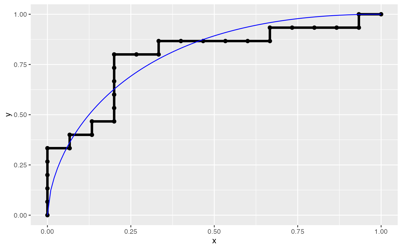
# See the fit through the fitted values
ggplot2::ggplot(rocxy, ggplot2::aes(x = x, y = y)) +
  geom_roc(shape = 19, size = 2) +
  geom_rocfit(data = rocxy, col = "blue")