Fit Weighted k-Nearest Neighbor Classifier

Wrapper for fitting weighted k-nearest neighbor classifiers.

Usage

fit_kknn(
  formula,
  train,
  test,
  k_neighbors = 10,
  distance = 2,
  kernel = "triangular",
  ...
)

Arguments

formula: A formula class object, specifying the model to be fitted (e.g. \(response ~ x_1 + x_2 + ... + x_n\)).
train: Matrix or data frame of training set cases.
test: Matrix or data frame of test set cases.
k_neighbors: See k in kknn::kknn().
distance: numeric(1). Parameter of Minkowski distance. Manhattan = 1 and Euclidean = 2.
kernel: Kernel to use. Possible choices are "rectangular" (which is standard unweighted knn), "triangular", "epanechnikov" (or beta(2,2)), "biweight" (or beta(3,3)), "triweight" (or beta(4,4)), "cos", "inv", "gaussian", "rank" and "optimal".
...: Additional arguments passed to kknn::kknn().

Value

A k-nearest neighbors model, as returned by kknn::kknn(), with a "Response" variable, classes, and function parameters train, k, distance, kernel, as well as the function call (call) added as entries to the list.

Author

Stu Field

Examples

# Use fake training data from iris data set
train_idx <- sample(nrow(tr_iris), 90L)  # random 90% training
test_df   <- tr_iris[-train_idx, ]
kknnfit   <- fit_kknn(Species ~ ., train = tr_iris[train_idx, ], test = test_df)
pos  <- get_pos_class(kknnfit)
pred <- calc_predictions(kknnfit) # internal test predictions
pred
#> # A tibble: 10 × 3
#>    pred_class prob_setosa prob_virginica
#>    <chr>            <dbl>          <dbl>
#>  1 virginica       0.314          0.686 
#>  2 setosa          0.522          0.478 
#>  3 virginica       0.155          0.845 
#>  4 setosa          0.593          0.407 
#>  5 setosa          0.709          0.291 
#>  6 setosa          0.672          0.328 
#>  7 virginica       0.445          0.555 
#>  8 setosa          0.956          0.0444
#>  9 virginica       0.0268         0.973 
#> 10 virginica       0.444          0.556 

# Confusion matrix
calc_confusion(test_df$Species, pred$prob_virginica, pos_class = pos) |>
  summary()
#> ══ Confusion Matrix Summary ═══════════════════════════════════════════
#> ── Confusion ──────────────────────────────────────────────────────────
#> 
#> Positive Class: virginica
#> 
#>            Predicted
#> Truth       setosa virginica
#>   setosa         3         2
#>   virginica      2         3
#> 
#> ── Performance Metrics (CI95%) ────────────────────────────────────────
#> 
#> # A tibble: 10 × 5
#>    metric              n estimate CI95_lower CI95_upper
#>    <chr>           <int>    <dbl>      <dbl>      <dbl>
#>  1 Sensitivity         5    0.6       0.110       1    
#>  2 Specificity         5    0.6       0.110       1    
#>  3 PPV (Precision)     5    0.6       0.110       1    
#>  4 NPV                 5    0.6       0.110       1    
#>  5 Accuracy           10    0.6       0.254       0.946
#>  6 Bal Accuracy       10    0.6       0.254       0.946
#>  7 Prevalence         10    0.5       0.146       0.854
#>  8 AUC                10    0.52      0.167       0.873
#>  9 Brier Score        10    0.370     0.0284      0.711
#> 10 MCC                NA    0.2      NA          NA    
#> 
#> ── Additional Statistics ──────────────────────────────────────────────
#> 
#> F_measure    G_mean    Wt_Acc 
#>       0.6       0.6       0.6 

# plot ROC
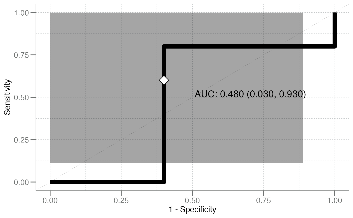
plot_emp_roc(test_df$Species, pred$prob_virginica, pos)
#> Warning: Using `size` aesthetic for lines was deprecated in ggplot2 3.4.0.
#> ℹ Please use `linewidth` instead.
#> ℹ The deprecated feature was likely used in the libml package.
#>   Please report the issue to the authors.
#> Warning: The `size` argument of `element_line()` is deprecated as of ggplot2
#> 3.4.0.
#> ℹ Please use the `linewidth` argument instead.
#> ℹ The deprecated feature was likely used in the libml package.
#>   Please report the issue to the authors.